
![]()
Version 0.97, June 2004
Authors of the program: Nicolas Brouard, senior researcher at the Institut National d'Etudes Démographiques (INED, Paris) in the "Mortality, Health and Epidemiology" Research Unit
and Agnès Lièvre
This program computes Healthy Life Expectancies from cross-longitudinal data using the methodology pioneered by Laditka and Wolf (1). Within the family of Health Expectancies (HE), disability-free life expectancy (DFLE) is probably the most important index to monitor. In low mortality countries, there is a fear that when mortality declines (and therefore total life expectancy improves), the increase will not be as great, leading to an Expansion of morbidity. Most of the data collected today, in particular by the international REVES network on Health Expectancy and the disability process, and most HE indices based on these data, are cross-sectional. This means that the information collected comes from a single cross-sectional survey: people from a variety of ages (but often old people) are surveyed on their health status at a single date. The proportion of people disabled at each age can then be estimated at that date. This age-specific prevalence curve is used to distinguish, within the stationary population (which, by definition, is the life table estimated from the vital statistics on mortality at the same date), the disabled population from the disability-free population. Life expectancy (LE) (or total population divided by the yearly number of births or deaths of this stationary population) is then decomposed into disability-free life expectancy (DFLE) and disability life expectancy (DLE). This method of computing HE is usually called the Sullivan method (after the author who first described it).
The age-specific proportions of people disabled (prevalence of disability) are dependent upon the historical flows from entering disability and recovering in the past. The age-specific forces (or incidence rates) of entering disability or recovering a good health, estimated over a recent period of time (as period forces of mortality), are reflecting current conditions and therefore can be used at each age to forecast the future of this cohort if nothing changes in the future, i.e to forecast the prevalence of disability of each cohort. Our finding (2) is that the period prevalence of disability (computed from period incidences) is lower than the cross-sectional prevalence. For example if a country is improving its technology of prosthesis, the incidence of recovering the ability to walk will be higher at each (old) age, but the prevalence of disability will only slightly reflect an improvement because the prevalence is mostly affected by the history of the cohort and not by recent period effects. To measure the period improvement we have to simulate the future of a cohort of new-borns entering or leaving the disability state or dying at each age according to the incidence rates measured today on different cohorts. The proportion of people disabled at each age in this simulated cohort will be much lower that the proportions observed at each age in a cross-sectional survey. This new prevalence curve introduced in a life table will give a more realistic HE level than the Sullivan method which mostly reflects the history of health conditions in a country.
Therefore, the main question is how can we measure incidence rates from cross-longitudinal surveys? This is the goal of the IMaCH program. From your data and using IMaCH you can estimate period HE as well as the Sullivan HE. In addition the standard errors of the HE are computed.
A cross-longitudinal survey consists of a first survey ("cross") where
individuals of different ages are interviewed about their health status or degree
of disability. At least a second wave of interviews ("longitudinal") should
measure each individual new health status. Health expectancies are computed from
the transitions observed between waves (interviews) and are computed for each degree of
severity of disability (number of health states). The more degrees of severity considered, the more
time is necessary to reach the Maximum Likelihood of the parameters involved in
the model. Considering only two states of disability (disabled and healthy) is
generally enough but the computer program works also with more health
states.
The simplest model for the transition probabilities is the multinomial logistic model where
pij is the probability to be observed in state j at the second
wave conditional to be observed in state i at the first wave. Therefore
a simple model is: log(pij/pii)= aij + bij*age+ cij*sex, where
'age' is age and 'sex' is a covariate. The advantage that this
computer program claims, is that if the delay between waves is not
identical for each individual, or if some individual missed an interview, the
information is not rounded or lost, but taken into account using an
interpolation or extrapolation. hPijx is the probability to be observed
in state i at age x+h conditional on the observed state i
at age x. The delay 'h' can be split into an exact number
(nh*stepm) of unobserved intermediate states. This elementary transition
(by month or quarter, trimester, semester or year) is modeled as the above multinomial
logistic. The hPx matrix is simply the matrix product of nh*stepm
elementary matrices and the contribution of each individual to the likelihood is
simply hPijx.
The program presented in this manual is a general program named
IMaCh (for Interpolated
MArkov CHain), designed to analyse transitions from longitudinal surveys. The first step is the estimation of the set of the parameters of a model for the
transition probabilities between an initial state and a final state.
From there, the computer program produces indicators such as the observed and
stationary prevalence, life expectancies and their variances both numerically and graphically. Our
transition model consists of absorbing and non-absorbing states assuming the
possibility of return across the non-absorbing states. The main advantage of
this package, compared to other programs for the analysis of transition data
(for example: Proc Catmod of SAS®) is that the whole individual
information is used even if an interview is missing, a state or a date is
unknown or when the delay between waves is not identical for each individual.
The program is dependent upon a set of parameters inputted by the user: selection of a sub-sample,
number of absorbing and non-absorbing states, number of waves to be taken in account , a tolerance level for the
maximization function, the periodicity of the transitions (we can compute
annual, quarterly or monthly transitions), covariates in the model. IMaCh works on
Windows or on Unix platform.
(1) Laditka S. B. and Wolf, D. (1998), New Methods for Analyzing Active Life Expectancy. Journal of Aging and Health. Vol 10, No. 2.
The minimum data required for a transition model is the recording of a set of individuals interviewed at a first date and interviewed once more. From the observations of an individual, we obtain a follow-up over time of the occurrence of a specific event. In this documentation, the event is related to health state, but the program can be applied to many longitudinal studies with different contexts. To build the data file as explained in the next section, you must have the month and year of each interview and the corresponding health state. In order to get age, date of birth (month and year) are required (missing values are allowed for month). Date of death (month and year) is an important information also required if the individual is dead. Shorter steps (i.e. a month) will more closely take into account the survival time after the last interview.
In this example, 8,000 people have been interviewed in a cross-longitudinal survey of 4 waves (1984, 1986, 1988, 1990). Some people missed 1, 2 or 3 interviews. Health states are healthy (1) and disabled (2). The survey is not a real one but a simulation of the American Longitudinal Survey on Aging. The disability state is defined as dependence in at least one of four ADLs (Activities of daily living, like bathing, eating, walking). Therefore, even if the individuals interviewed in the sample are virtual, the information in this sample is close to reality for the United States. Sex is not recorded is this sample. The LSOA survey is biased in the sense that people living in an institution were not included in the first interview in 1984. Thus the prevalence of disability observed in 1984 is lower than the true prevalence at old ages. However when people moved into an institution, they were interviewed there in 1986, 1988 and 1990. Thus the incidences of disabilities are not biased. Cross-sectional prevalences of disability at old ages are thus artificially increasing in 1986, 1988 and 1990 because of a greater proportion of the sample institutionalized. Our article (Lièvre A., Brouard N. and Heathcote Ch. (2003)) shows the opposite: the period prevalence based on the incidences is lower at old ages than the adjusted cross-sectional prevalence illustrating that there has been significant progress against disability.
Each line of the data set (named data1.txt in this first example) is an individual record. Fields are separated by blanks:
If you do not wish to include information on weights or covariates, you must fill the column with a number (e.g. 1) since all fields must be present.
This first line was a comment. Comments line start with a '#'.
title=1st_example datafile=data1.txt lastobs=8600 firstpass=1 lastpass=4
ftol=1.e-08 stepm=1 ncovcol=2 nlstate=2 ndeath=1 maxwav=4 mle=1 weight=0
Intercept and age are automatically included in the model. Additional covariates can be included with the command:
model=list of covariates
In this example, we have two covariates in the data file (fields 2 and 3). The number of covariates included in the data file between the id and the date of birth is ncovcol=2 (it was named ncov in version prior to 0.8). If you have 3 covariates in the datafile (fields 2, 3 and 4), you will set ncovcol=3. Then you can run the programme with a new parametrisation taking into account the third covariate. For example, model=V1+V3 estimates a model with the first and third covariates. More complicated models can be used, but this will take more time to converge. With a simple model (no covariates), the programme estimates 8 parameters. Adding covariates increases the number of parameters : 12 for model=V1, 16 for model=V1+V1*age and 20 for model=V1+V2+V3.
You must write the initial guess values of the parameters for optimization.
The number of parameters, N depends on the number of absorbing states
and non-absorbing states and on the number of covariates in the model (ncovmodel).
N is
given by the formula N=(nlstate +
ndeath-1)*nlstate*ncovmodel .
Thus in
the simple case with 2 covariates in the model(the model is log (pij/pii) = aij + bij * age
where intercept and age are the two covariates), and 2 health states (1 for
disability-free and 2 for disability) and 1 absorbing state (3), you must enter
8 initials values, a12, b12, a13, b13, a21, b21, a23, b23. You can start with
zeros as in this example, but if you have a more precise set (for example from
an earlier run) you can enter it and it will speed up the convergence
Each of the four
lines starts with indices "ij": ij aij bij
# Guess values of aij and bij in log (pij/pii) = aij + bij * age
12 -14.155633  0.110794
13  -7.925360  0.032091
21  -1.890135 -0.029473
23  -6.234642  0.022315
or, to simplify (in most of cases it converges but there is no warranty!):
12 0.0 0.0
13 0.0 0.0
21 0.0 0.0
23 0.0 0.0
In order to speed up the convergence you can make a first run with a large stepm i.e stepm=12 or 24 and then decrease the stepm until stepm=1 month. If newstepm is the new shorter stepm and stepm can be expressed as a multiple of newstepm, like newstepm=n stepm, then the following approximation holds:
aij(stepm) = aij(n . stepm) - ln(n)
and
bij(stepm) = bij(n . stepm) .
For example if you already ran with stepm=6 (a 6 months interval) and got:
# Parameters
12 -13.390179  0.126133
13  -7.493460  0.048069
21   0.575975 -0.041322
23  -4.748678  0.030626
Then you now want to get the monthly estimates, you can guess the aij by
subtracting ln(6)= 1.7917
and running using
12 -15.18193847  0.126133
13 -9.285219469  0.048069
21 -1.215784469 -0.041322
23 -6.540437469  0.030626
and get
12 -15.029768 0.124347 13 -8.472981 0.036599 21 -1.472527 -0.038394 23 -6.553602 0.029856which is closer to the results. The approximation is probably useful only for very small intervals and we don't have enough experience to know if you will speed up the convergence or not.
         -ln(12)= -2.484
 -ln(6/1)=-ln(6)= -1.791
 -ln(3/1)=-ln(3)= -1.0986
-ln(12/6)=-ln(2)= -0.693
In version 0.9 and higher you can still have valuable results even if your stepm parameter is bigger than a month. The idea is to run with bigger stepm in order to have a quicker convergence at the price of a small bias. Once you know which model you want to fit, you can put stepm=1 and wait hours or days to get the convergence! To get unbiased results even with large stepm we introduce the idea of pseudo likelihood by interpolating two exact likelihoods. In more detail:
If the interval of d months between two waves is not a multiple of
'stepm', but is between (n-1) stepm and n stepm then
both exact likelihoods are computed (the contribution to the likelihood at n
stepm requires one matrix product more) (let us remember that we are
modelling the probability to be observed in a particular state after d
months being observed at a particular state at 0). The distance, (bh in
the program), from the month of interview to the rounded date of n
stepm is computed. It can be negative (interview occurs before n
stepm) or positive if the interview occurs after n stepm (and
before (n+1)stepm).
Then the final contribution to the total
likelihood is a weighted average of these two exact likelihoods at n
stepm (out) and at (n-1)stepm(savm). We did not want to compute
the third likelihood at (n+1)stepm because it is too costly in time, so
we used an extrapolation if bh is positive.
The formula
for the inter/extrapolation may vary according to the value of parameter mle:
mle=1	  lli= log((1.+bbh)*out[s1][s2]- bbh*savm[s1][s2]); /* linear interpolation */

mle=2	lli= (savm[s1][s2]>(double)1.e-8 ? \
          log((1.+bbh)*out[s1][s2]- bbh*(savm[s1][s2])): \
          log((1.+bbh)*out[s1][s2])); /* linear interpolation */
mle=3	lli= (savm[s1][s2]>1.e-8 ? \
          (1.+bbh)*log(out[s1][s2])- bbh*log(savm[s1][s2]): \
          log((1.+bbh)*out[s1][s2])); /* exponential inter-extrapolation */

mle=4   lli=log(out[s[mw[mi][i]][i]][s[mw[mi+1][i]][i]]); /* No interpolation  */
        no need to save previous likelihood into memory.
If the death occurs between the first and second pass, and for example more precisely between n stepm and (n+1)stepm the contribution of these people to the likelihood is simply the difference between the probability of dying before n stepm and the probability of dying before (n+1)stepm. There was a bug in version 0.8 and death was treated as any other state, i.e. as if it was an observed death at second pass. This was not precise but correct, although when information on the precise month of death came (death occuring prior to second pass) we did not change the likelihood accordingly. We thank Chris Jackson for correcting it. In earlier versions (fortunately before first publication) the total mortality was thus overestimated (people were dying too early) by about 10%. Version 0.95 and higher are correct.
Our suggested choice is mle=1 . If stepm=1 there is no difference between various mle options (methods of interpolation). If stepm is big, like 12 or 24 or 48 and mle=4 (no interpolation) the bias may be very important if the mean duration between two waves is not a multiple of stepm. See the appendix in our main publication concerning the sine curve of biases.
These values are output by the maximisation of the likelihood mle=1 and can be used as an input for a second run in order to get the various output data files (Health expectancies, period prevalence etc.) and figures without rerunning the long maximisation phase (mle=0).
The 'scales' are small values needed for the computing of numerical derivatives. These derivatives are used to compute the hessian matrix of the parameters, that is the inverse of the covariance matrix. They are often used for estimating variances and confidence intervals. Each line consists of indices "ij" followed by the initial scales (zero to simplify) associated with aij and bij.
# Scales (for hessian or gradient estimation)
12 0. 0.
13 0. 0.
21 0. 0.
23 0. 0.
The covariance matrix is output if mle=1. But it can be
also be used as an input to get the various output data files (Health
expectancies, period prevalence etc.) and figures without rerunning
the maximisation phase (mle=0).
Each line starts with indices
"ijk" followed by the covariances between aij and bij:
   121 Var(a12)
   122 Cov(b12,a12)  Var(b12)
          ...
   232 Cov(b23,a12)  Cov(b23,b12) ... Var (b23)
# Covariance matrix
121 0.
122 0. 0.
131 0. 0. 0.
132 0. 0. 0. 0.
211 0. 0. 0. 0. 0.
212 0. 0. 0. 0. 0. 0.
231 0. 0. 0. 0. 0. 0. 0.
232 0. 0. 0. 0. 0. 0. 0. 0.
agemin=70 agemax=100 bage=50 fage=100
Once we obtained the estimated parameters, the program is able to calculate period prevalence, transitions probabilities and life expectancies at any age. Choice of the age range is useful for extrapolation. In this example, the age of people interviewed varies from 69 to 102 and the model is estimated using their exact ages. But if you are interested in the age-specific period prevalence you can start the simulation at an exact age like 70 and stop at 100. Then the program will draw at least two curves describing the forecasted prevalences of two cohorts, one for healthy people at age 70 and the second for disabled people at the same initial age. And according to the mixing property (ergodicity) and because of recovery, both prevalences will tend to be identical at later ages. Thus if you want to compute the prevalence at age 70, you should enter a lower agemin value.
Setting bage=50 (begin age) and fage=100 (final age), let the program compute life expectancy from age 'bage' to age 'fage'. As we use a model, we can interessingly compute life expectancy on a wider age range than the age range from the data. But the model can be rather wrong on much larger intervals. Program is limited to around 120 for upper age!
begin-prev-date=1/1/1984 end-prev-date=1/6/1988 estepm=1
Statements 'begin-prev-date' and 'end-prev-date' allow the user to select the period in which the observed prevalences in each state. In this example, the prevalences are calculated on data survey collected between 1 January 1984 and 1 June 1988.
pop_based=0
The program computes status-based health expectancies, i.e health
expectancies which depend on the initial health state. If you are healthy, your
healthy life expectancy (e11) is higher than if you were disabled (e21, with e11
> e21).
To compute a healthy life expectancy 'independent' of the initial
status we have to weight e11 and e21 according to the probability of
being in each state at initial age which correspond to the proportions
of people in each health state (cross-sectional prevalences).
We could also compute e12 and e12 and get e.2 by weighting them according to the observed cross-sectional prevalences at initial age.
In a similar way we could compute the total life expectancy by summing e.1
and e.2 .
The main difference between 'population based' and 'implied' or
'period' is in the weights used. 'Usually', cross-sectional prevalences of
disability are higher than period prevalences particularly at old ages. This is
true if the country is improving its health system by teaching people how to
prevent disability by promoting better screening, for example of people
needing cataract surgery. Then the proportion of disabled people at
age 90 will be lower than the current observed proportion.
Thus a better Health Expectancy and even a better Life Expectancy value is
given by forecasting not only the current lower mortality at all ages but also a
lower incidence of disability and higher recovery.
Using the period
prevalences as weight instead of the cross-sectional prevalences we are
computing indices which are more specific to the current situations and
therefore more useful to predict improvements or regressions in the future as to
compare different policies in various countries.
starting-proj-date=1/1/1989 final-proj-date=1/1/1992 mov_average=0
Prevalence and population projections are only available if the interpolation
unit is a month, i.e. stepm=1 and if there are no covariate. The programme
estimates the prevalence in each state at a precise date expressed in
day/month/year. The programme computes one forecasted prevalence a year from a
starting date (1 January 1989 in this example) to a final date (1 January
1992). The statement mov_average allows computation of smoothed forecasted
prevalences with a five-age moving average centered at the mid-age of the
fiveyear-age period.
We assume that you have already typed your 1st_example parameter file as explained above. To run the program under Windows you should either:
The time to converge depends on the step unit used (1 month is more precise but more cpu time consuming), on the number of cases, and on the number of variables (covariates).
The program outputs many files. Most of them are files which will be plotted for better understanding.
To run under Linux is mostly the same.It is no more difficult to run IMaCh on a MacIntosh.
Once the optimization is finished (once the convergence is reached), many tables and graphics are produced.
The IMaCh program will create a subdirectory with the same name as your
parameter file (here mypar) where all the tables and figures will be
stored.
Important files like the log file and the output parameter file
(the latter contains the maximum likelihood estimates) are stored at
the main level not in this subdirectory. Files with extension .log and
.txt can be edited with a standard editor like wordpad or notepad or
even can be viewed with a browser like Internet Explorer or Mozilla.
The main html file is also named with the same name biaspar.htm. You can click on it by holding your shift key in order to open it in another window (Windows).
Our grapher is Gnuplot, an interactive plotting program (GPL) which can
also work in batch mode. A gnuplot reference manual is available here.
When the run is finished, and in
order that the window doesn't disappear, the user should enter a character like
q for quitting.
These characters are:
Gnuplot is easy and you can use it to make more complex graphs. Just click on gnuplot and type plot sin(x) to see how easy it is.
The first line is the title and displays each field of the file. First column
corresponds to age. Fields 2 and 6 are the proportion of individuals in states 1
and 2 respectively as observed at first exam. Others fields are the numbers of
people in states 1, 2 or more. The number of columns increases if the number of
states is higher than 2.
The header of the file is
# Age Prev(1) N(1) N Age Prev(2) N(2) N
70 1.00000 631 631 70 0.00000 0 631
71 0.99681 625 627 71 0.00319 2 627
72 0.97125 1115 1148 72 0.02875 33 1148
It means that at age 70 (between 70 and 71), the prevalence in state 1 is
1.000 and in state 2 is 0.00 . At age 71 the number of individuals in state 1 is
625 and in state 2 is 2, hence the total number of people aged 71 is 625+2=627.
This file contains all the maximisation results:
 -2 log likelihood= 21660.918613445392
 Estimated parameters: a12 = -12.290174 b12 = 0.092161
                       a13 = -9.155590  b13 = 0.046627
                       a21 = -2.629849  b21 = -0.022030
                       a23 = -7.958519  b23 = 0.042614
 Covariance matrix: Var(a12) = 1.47453e-001
                    Var(b12) = 2.18676e-005
                    Var(a13) = 2.09715e-001
                    Var(b13) = 3.28937e-005
                    Var(a21) = 9.19832e-001
                    Var(b21) = 1.29229e-004
                    Var(a23) = 4.48405e-001
                    Var(b23) = 5.85631e-005
By substitution of these parameters in the regression model, we obtain the elementary transition probabilities:
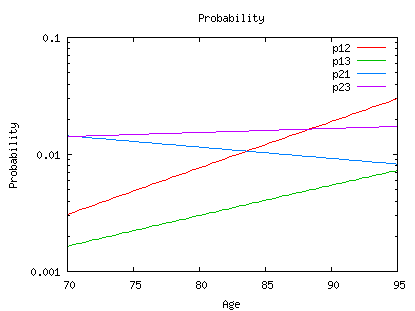
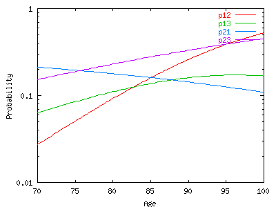
Here are the transitions probabilities Pij(x, x+nh). The second column is the starting age x (from age 95 to 65), the third is age (x+nh) and the others are the transition probabilities p11, p12, p13, p21, p22, p23. The first column indicates the value of the covariate (without any other variable than age it is equal to 1) For example, line 5 of the file is:
1 100 106 0.02655 0.17622 0.79722 0.01809 0.13678 0.84513
and this means:
p11(100,106)=0.02655
p12(100,106)=0.17622
p13(100,106)=0.79722
p21(100,106)=0.01809
p22(100,106)=0.13678
p22(100,106)=0.84513
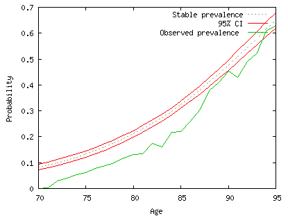
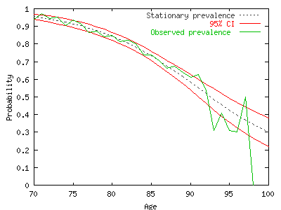
#Prevalence
#Age 1-1 2-2

#************
70 0.90134 0.09866
71 0.89177 0.10823
72 0.88139 0.11861
73 0.87015 0.12985
At age 70 the period prevalence is 0.90134 in state 1 and 0.09866 in state 2. This period prevalence differs from the cross-sectional prevalence and we explaining. The cross-sectional prevalence at age 70 results from the incidence of disability, incidence of recovery and mortality which occurred in the past for the cohort. Period prevalence results from a simulation with current incidences of disability, recovery and mortality estimated from this cross-longitudinal survey. It is a good prediction of the prevalence in the future if "nothing changes in the future". This is exactly what demographers do with a period life table. Life expectancy is the expected mean survival time if current mortality rates (age-specific incidences of mortality) "remain constant" in the future.
The period prevalence has to be compared with the cross-sectional prevalence.
But both are statistical estimates and therefore have confidence intervals.
For the cross-sectional prevalence we generally need information on the
design of the surveys. It is usually not enough to consider the number of people
surveyed at a particular age and to estimate a Bernouilli confidence interval
based on the prevalence at that age. But you can do it to have an idea of the
randomness. At least you can get a visual appreciation of the randomness by
looking at the fluctuation over ages.
For the period prevalence it is possible to estimate the confidence interval from the Hessian matrix (see the publication for details). We are supposing that the design of the survey will only alter the weight of each individual. IMaCh scales the weights of individuals-waves contributing to the likelihood by making the sum of the weights equal to the sum of individuals-waves contributing: a weighted survey doesn't increase or decrease the size of the survey, it only give more weight to some individuals and thus less to the others.
This graph exhibits the period prevalence in state (2) with the confidence interval in red. The green curve is the observed prevalence (or proportion of individuals in state (2)). Without discussing the results (it is not the purpose here), we observe that the green curve is somewhat below the period prevalence. If the data were not biased by the non inclusion of people living in institutions we would have concluded that the prevalence of disability will increase in the future (see the main publication if you are interested in real data and results which are opposite).
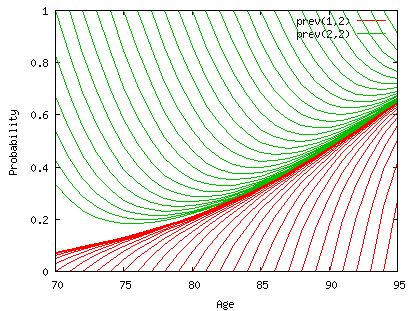
This graph plots the conditional transition probabilities from an initial state (1=healthy in red at the bottom, or 2=disabled in green on the top) at age x to the final state 2=disabled at age x+h where conditional means conditional on being alive at age x+h which is hP12x + hP22x. The curves hP12x/(hP12x + hP22x) and hP22x/(hP12x + hP22x) converge with h, to the period prevalence of disability. In order to get the period prevalence at age 70 we should start the process at an earlier age, i.e.50. If the disability state is defined by severe disability criteria with only a small chance of recovering, then the incidence of recovery is low and the time to convergence is probably longer. But we don't have experience of this yet.
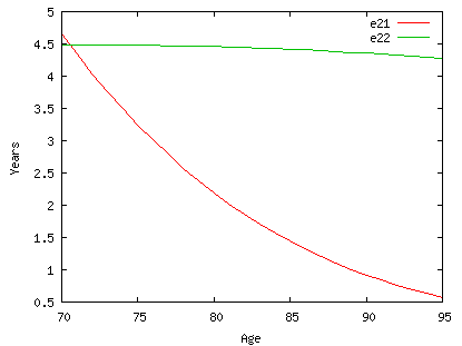
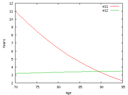
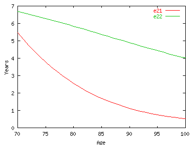
# Health expectancies
# Age 1-1 (SE) 1-2 (SE) 2-1 (SE) 2-2 (SE)
 70   11.0180 (0.1277)    3.1950 (0.3635)    4.6500 (0.0871)    4.4807 (0.2187)
 71   10.4786 (0.1184)    3.2093 (0.3212)    4.3384 (0.0875)    4.4820 (0.2076)
 72    9.9551 (0.1103)    3.2236 (0.2827)    4.0426 (0.0885)    4.4827 (0.1966)
 73    9.4476 (0.1035)    3.2379 (0.2478)    3.7621 (0.0899)    4.4825 (0.1858)
 74    8.9564 (0.0980)    3.2522 (0.2165)    3.4966 (0.0920)    4.4815 (0.1754)
 75    8.4815 (0.0937)    3.2665 (0.1887)    3.2457 (0.0946)    4.4798 (0.1656)
 76    8.0230 (0.0905)    3.2806 (0.1645)    3.0090 (0.0979)    4.4772 (0.1565)
 77    7.5810 (0.0884)    3.2946 (0.1438)    2.7860 (0.1017)    4.4738 (0.1484)
 78    7.1554 (0.0871)    3.3084 (0.1264)    2.5763 (0.1062)    4.4696 (0.1416)
 79    6.7464 (0.0867)    3.3220 (0.1124)    2.3794 (0.1112)    4.4646 (0.1364)
 80    6.3538 (0.0868)    3.3354 (0.1014)    2.1949 (0.1168)    4.4587 (0.1331)
 81    5.9775 (0.0873)    3.3484 (0.0933)    2.0222 (0.1230)    4.4520 (0.1320)
For example  70  11.0180 (0.1277) 3.1950 (0.3635) 4.6500 (0.0871)  4.4807 (0.2187)
means
e11=11.0180 e12=3.1950 e21=4.6500 e22=4.4807
For example, life expectancy of a healthy individual at age 70 is 11.0 in the healthy state and 3.2 in the disability state (total of 14.2 years). If he was disabled at age 70, his life expectancy will be shorter, 4.65 years in the healthy state and 4.5 in the disability state (=9.15 years). The total life expectancy is a weighted mean of both, 14.2 and 9.15. The weight is the proportion of people disabled at age 70. In order to get a period index (i.e. based only on incidences) we use the stable or period prevalence at age 70 (i.e. computed from incidences at earlier ages) instead of the cross-sectional prevalence (observed for example at first interview) (see below).
For example, the covariances of life expectancies Cov(ei,ej) at age 50 are (line 3)
Cov(e1,e1)=0.4776 Cov(e1,e2)=0.0488=Cov(e2,e1) Cov(e2,e2)=0.0424
For example, at age 65
p11=9.960e-001 standard deviation of p11=2.359e-004
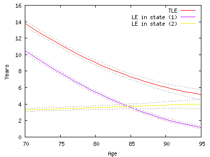
#Total LEs with variances: e.. (std) e.1 (std) e.2 (std)
70 13.26 (0.22) 9.95 (0.20) 3.30 (0.14)
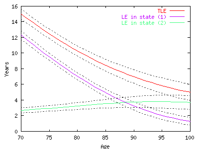
Thus, at age 70 the total life expectancy, e..=13.26 years is the weighted mean of e1.=13.46 and e2.=11.35 by the period prevalences at age 70 which are 0.90134 in state 1 and 0.09866 in state 2 respectively (the sum is equal to one). e.1=9.95 is the Disability-free life expectancy at age 70 (it is again a weighted mean of e11 and e21). e.2=3.30 is also the life expectancy at age 70 to be spent in the disability state.
This figure represents the health expectancies and the total life expectancy with a confidence interval (dashed line).
Standard deviations (obtained from the information matrix of the model) of these quantities are very useful. Cross-longitudinal surveys are costly and do not involve huge samples, generally a few thousands; therefore it is very important to have an idea of the standard deviation of our estimates. It has been a big challenge to compute the Health Expectancy standard deviations. Don't be confused: life expectancy is, as any expected value, the mean of a distribution; but here we are not computing the standard deviation of the distribution, but the standard deviation of the estimate of the mean.
Our health expectancy estimates vary according to the sample size (and the standard deviations give confidence intervals of the estimates) but also according to the model fitted. We explain this in more detail.
Choosing a model means at least two kind of choices. First we have to decide the number of disability states. And second we have to design, within the logit model family, the model itself: variables, covariates, confounding factors etc. to be included.
The more disability states we have, the better is our demographical approximation of the disability process, but the smaller the number of transitions between each state and the higher the noise in the measurement. We have not experimented enough with the various models to summarize the advantages and disadvantages, but it is important to note that even if we had huge unbiased samples, the total life expectancy computed from a cross-longitudinal survey would vary with the number of states. If we define only two states, alive or dead, we find the usual life expectancy where it is assumed that at each age, people are at the same risk of dying. If we are differentiating the alive state into healthy and disabled, and as mortality from the disabled state is higher than mortality from the healthy state, we are introducing heterogeneity in the risk of dying. The total mortality at each age is the weighted mean of the mortality from each state by the prevalence of each state. Therefore if the proportion of people at each age and in each state is different from the period equilibrium, there is no reason to find the same total mortality at a particular age. Life expectancy, even if it is a very useful tool, has a very strong hypothesis of homogeneity of the population. Our main purpose is not to measure differential mortality but to measure the expected time in a healthy or disabled state in order to maximise the former and minimize the latter. But the differential in mortality complicates the measurement.
Incidences of disability or recovery are not affected by the number of states if these states are independent. But incidence estimates are dependent on the specification of the model. The more covariates we add in the logit model the better is the model, but some covariates are not well measured, some are confounding factors like in any statistical model. The procedure to "fit the best model' is similar to logistic regression which itself is similar to regression analysis. We haven't yet been sofar because we also have a severe limitation which is the speed of the convergence. On a Pentium III, 500 MHz, even the simplest model, estimated by month on 8,000 people may take 4 hours to converge. Also, the IMaCh program is not a statistical package, and does not allow sophisticated design variables. If you need sophisticated design variable you have to them your self and and add them as ordinary variables. IMaCh allows up to 8 variables. The current version of this program allows only to add simple variables like age+sex or age+sex+ age*sex but will never be general enough. But what is to remember, is that incidences or probability of change from one state to another is affected by the variables specified into the model.
Also, the age range of the people interviewed is linked the age range of the life expectancy which can be estimated by extrapolation. If your sample ranges from age 70 to 95, you can clearly estimate a life expectancy at age 70 and trust your confidence interval because it is mostly based on your sample size, but if you want to estimate the life expectancy at age 50, you should rely in the design of your model. Fitting a logistic model on a age range of 70 to 95 and estimating probabilties of transition out of this age range, say at age 50, is very dangerous. At least you should remember that the confidence interval given by the standard deviation of the health expectancies, are under the strong assumption that your model is the 'true model', which is probably not the case outside the age range of your sample.
This copy of the parameter file can be useful to re-run the program while saving the old output files.
First, we have estimated the observed prevalence between 1/1/1984 and 1/6/1988 (June, European syntax of dates). The mean date of all interviews (weighted average of the interviews performed between 1/1/1984 and 1/6/1988) is estimated to be 13/9/1985, as written on the top on the file. Then we forecast the probability to be in each state.
For example on 1/1/1989 :
# StartingAge FinalAge P.1 P.2 P.3
# Forecasting at date 1/1/1989
  73 0.807 0.078 0.115
Since the minimum age is 70 on the 13/9/1985, the youngest forecasted age is 73. This means that at age a person aged 70 at 13/9/1989 has a probability to enter state1 of 0.807 at age 73 on 1/1/1989. Similarly, the probability to be in state 2 is 0.078 and the probability to die is 0.115. Then, on the 1/1/1989, the prevalence of disability at age 73 is estimated to be 0.088.
# Age P.1 P.2 P.3 [Population]
# Forecasting at date 1/1/1989
75 572685.22 83798.08
74 621296.51 79767.99
73 645857.70 69320.60
# Forecasting at date 1/1/19909
76 442986.68 92721.14 120775.48
75 487781.02 91367.97 121915.51
74 512892.07 85003.47 117282.76
From the population file, we estimate the number of people in each state. At age 73, 645857 persons are in state 1 and 69320 are in state 2. One year latter, 512892 are still in state 1, 85003 are in state 2 and 117282 died before 1/1/1990.
Since you know how to run the program, it is time to test it on your own computer. Try for example on a parameter file named imachpar.imach which is a copy of mypar.imach included in the subdirectory of imach, mytry. Edit it and change the name of the data file to mydata.txt if you don't want to copy it on the same directory. The file mydata.txt is a smaller file of 3,000 people but still with 4 waves.
Right click on the .imach file and a window will popup with the string 'Enter the parameter file name:'
| IMACH, Version 0.97b
Enter the parameter file name: imachpar.imach |
Most of the data files or image files generated, will use the 'imachpar' string into their name. The running time is about 2-3 minutes on a Pentium III. If the execution worked correctly, the outputs files are created in the current directory, and should be the same as the mypar files initially included in the directory mytry.
Output on the screen The output screen looks like biaspar.log
#
title=MLE datafile=mydaiata.txt lastobs=3000 firstpass=1 lastpass=3
ftol=1.000000e-008 stepm=24 ncovcol=2 nlstate=2 ndeath=1 maxwav=4 mle=1 weight=0
Total number of individuals= 2965, Agemin = 70.00, Agemax= 100.92

Warning, no any valid information for:126 line=126
Warning, no any valid information for:2307 line=2307
Delay (in months) between two waves Min=21 Max=51 Mean=24.495826
These lines give some warnings on the data file and also some raw statistics on frequencies of transitions.
Age 70 1.=230 loss[1]=3.5% 2.=16 loss[2]=12.5% 1.=222 prev[1]=94.1% 2.=14
 prev[2]=5.9% 1-1=8 11=200 12=7 13=15 2-1=2 21=6 22=7 23=1
Age 102 1.=0 loss[1]=NaNQ% 2.=0 loss[2]=NaNQ% 1.=0 prev[1]=NaNQ% 2.=0
If you survey suffers from severe attrition, you have to analyse the characteristics of the lost people and overweight people with same characteristics for example.
By default, IMaCH warns and excludes these problematic people, but you have to be careful with such results.
Calculation of the hessian matrix. Wait...
12345678.12.13.14.15.16.17.18.23.24.25.26.27.28.34.35.36.37.38.45.46.47.48.56.57.58.67.68.78

Inverting the hessian to get the covariance matrix. Wait...

#Hessian matrix#
3.344e+002 2.708e+004 -4.586e+001 -3.806e+003 -1.577e+000 -1.313e+002 3.914e-001 3.166e+001
2.708e+004 2.204e+006 -3.805e+003 -3.174e+005 -1.303e+002 -1.091e+004 2.967e+001 2.399e+003
-4.586e+001 -3.805e+003 4.044e+002 3.197e+004 2.431e-002 1.995e+000 1.783e-001 1.486e+001
-3.806e+003 -3.174e+005 3.197e+004 2.541e+006 2.436e+000 2.051e+002 1.483e+001 1.244e+003
-1.577e+000 -1.303e+002 2.431e-002 2.436e+000 1.093e+002 8.979e+003 -3.402e+001 -2.843e+003
-1.313e+002 -1.091e+004 1.995e+000 2.051e+002 8.979e+003 7.420e+005 -2.842e+003 -2.388e+005
3.914e-001 2.967e+001 1.783e-001 1.483e+001 -3.402e+001 -2.842e+003 1.494e+002 1.251e+004
3.166e+001 2.399e+003 1.486e+001 1.244e+003 -2.843e+003 -2.388e+005 1.251e+004 1.053e+006
# Scales
12 1.00000e-004 1.00000e-006
13 1.00000e-004 1.00000e-006
21 1.00000e-003 1.00000e-005
23 1.00000e-004 1.00000e-005
# Covariance
  1 5.90661e-001
  2 -7.26732e-003 8.98810e-005
  3 8.80177e-002 -1.12706e-003 5.15824e-001
  4 -1.13082e-003 1.45267e-005 -6.50070e-003 8.23270e-005
  5 9.31265e-003 -1.16106e-004 6.00210e-004 -8.04151e-006 1.75753e+000
  6 -1.15664e-004 1.44850e-006 -7.79995e-006 1.04770e-007 -2.12929e-002 2.59422e-004
  7 1.35103e-003 -1.75392e-005 -6.38237e-004 7.85424e-006 4.02601e-001 -4.86776e-003 1.32682e+000
  8 -1.82421e-005 2.35811e-007 7.75503e-006 -9.58687e-008 -4.86589e-003 5.91641e-005 -1.57767e-002 1.88622e-004
# agemin agemax for lifexpectancy, bage fage (if mle==0 ie no data nor Max likelihood).


agemin=70 agemax=100 bage=50 fage=100
Computing prevalence limit: result on file 'plrmypar.txt'
Computing pij: result on file 'pijrmypar.txt'
Computing Health Expectancies: result on file 'ermypar.txt'
Computing Variance-covariance of DFLEs: file 'vrmypar.txt'
Computing Total LEs with variances: file 'trmypar.txt'
Computing Variance-covariance of Prevalence limit: file 'vplrmypar.txt'
End of Imach
Once the running is finished, the program requires a character:
| Type e to edit output files, g to graph again, c to start again, and q for exiting: |
First you should enter e to edit the master file mypar.htm.
This software have been partly granted by Euro-REVES, a concerted action from the European Union. Since 2003 it is also partly granted by the French Institute on Longevity. It will be copyrighted identically to a GNU software product, i.e. program and software can be distributed freely for non commercial use. Sources are not widely distributed today because some part of the codes are copyrighted by Numerical Recipes in C. You can get them by asking us with a simple justification (name, email, institute) mailto:brouard@ined.fr and mailto:lievre@ined.fr .
Latest version (0.97b of June 2004) can be accessed at http://euroreves.ined.fr/imach